Command palette
error Error

Pioneering AI for system control and coordination

1 • Why use AI for system control

Hjarl solves constrained, non-convex optimization

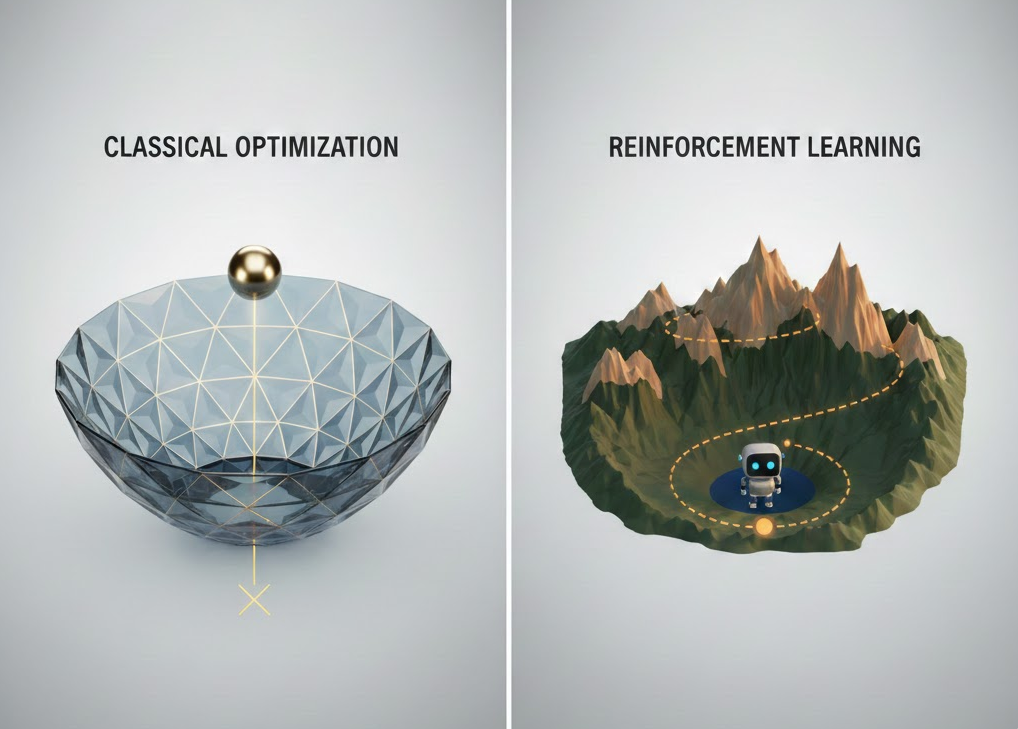
TODAY · TRIANGULATION ON CONVEX PROXY
HJARL · EXPLORATION OF REAL SURFACE
Exact solution to an imperfect representationlocal minimumx* (π*, λ*)Imperfect solution to a near-exact representation
THE CLASSICAL SOLUTION · MPC / SDDP
  • Exact solution to an imperfect representation: Linearizes equipment curves and constraints into a convex bowl.
  • Strict modeling rules: Requires simplifying assumptions on dynamics and uncertainty.
  • Hard to combine: Coupling adjacent systems rarely yields a convex problem.
THE HJARL APPROACH · NON-LINEAR PHYSICS
  • Imperfect solution to a near-exact representation: Captures non-linear dynamics, arbitrary distributions, and coupled systems.
  • Complementary and improvable: Benchmarks alongside classical solvers and improves through iterative training.
  • Testable optimum: Gradients (\nabla f) and shadow prices (\lambda^*) show what drives every action and how close a policy is to the optimum.

2 • Hjarl's offering

Local control over time, coordinated by signals in space

● agents optimize control locally
● coordination done over shadow prices
OPTIMAL CONTROL · LOCAL DOMAINS OVER TIME
  • Each policy optimizes control in its local domain over time and within hard limits.
  • Pilots: Hydropower reservoir dispatch & direct air capture process control.
  • Proof of concept: District heating boiler & storage control.
OPTIMAL SIGNALS · COORDINATION IN SPACE (IN R&D)
  • Shadow price signals pass up and down the hierarchy so local decisions align with the global optimum.
  • Showcase: Nodal shadow pricing in AC power grids.

3 • The Hjarl trinity

⅓ Engineering • ⅓ AI • ⅓ Optimization

∇fπ*λ*
● causal sampling (π* → ∇f → λ*)
● causal learning (∇f → π* → λ*)
∇f • Differentiable simulator

Modular physics components run forward while exact gradients pass backward through time, replacing trial-and-error sampling.

π* • Learned decision policy

Maps live system states and external drivers to control setpoints. Once trained, inference is immediate.

λ* • Equilibrium solver

Updates control policies and constraint shadow prices (λ*) together so the system converges within hard physical limits.

NOT A BLACK BOX

Every decision is traceable through exact gradients and shadow prices.

4 • Not just for operators

For live advice, performance benchmarks, and system design

operator > agent → refine simulatoragent > operator → upgrade procedure
1 • Advise live operations

Read live state tags and return recommended setpoints and sensitivities as operating conditions shift.

2 • Benchmark operator and policy

Where the operator outperforms the policy, refine the simulator; where the policy outperforms, improve operating procedures.

3 • Co-optimize designs and policies

Treat physical design parameters as trainable variables alongside the control policy to size and configure systems before committing capital.

5 • Path to running live · Removr / Honeywell DAC pilot

From simulator to sandboxed deployment

1 • Model the physics

Assembled a transient thermodynamic simulator with adsorption hysteresis and kinetics transients.

2 • Train in parallel

Trained the policy for 400M simulated hours (10,000 × 40,000h batches) across weather, power price, and CO₂ price regimes.

3 • Benchmark and run in a sandbox

Demonstrated meaningful economic uplift against the default operating policy, then deployed on a sandboxed server advising the Honeywell control system.

Example use cases

🌊 Hydropower dispatch

💨 Direct air capture

⚡ AC power grids

🏭 District heating

Optimal control use cases

🌊 Hydropower dispatch: Resource allocation under uncertainty

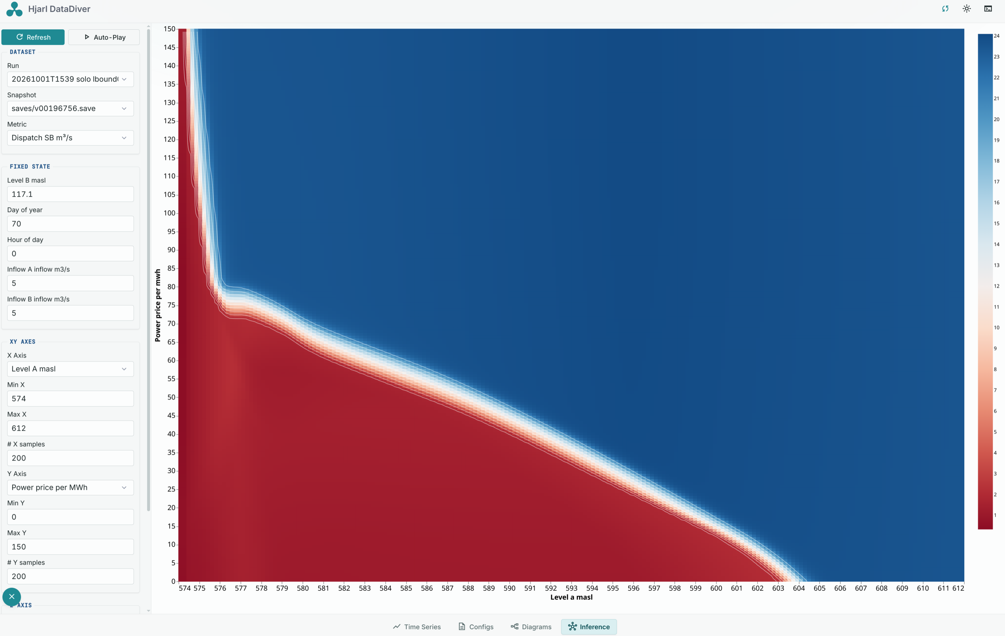
DISPATCH POLICY SENSITIVITY
Hydropower dispatch
PILOT · SKAGERAK ENERGI

Modular waterway, generator, reservoir, and spillway simulator training constrained dispatch policies and terminal values (yielding reservoir water values ∂V/∂W) across >1-year horizons.

BEYOND CONVEX PROXIES (SDDP)

Avoids SDDP's simplifying assumptions on inflow distributions, price dynamics, and head dynamics - optimizing across multiple end markets with immediate inference.
EXTENSIBLE ACROSS COUPLED ASSETS
  • Co-optimization with batteries, pumping, and industrial loads.
  • Load-based grid tariffs.

Optimal control use cases

💨 Carbon direct air capture: Thermodynamic process optimization

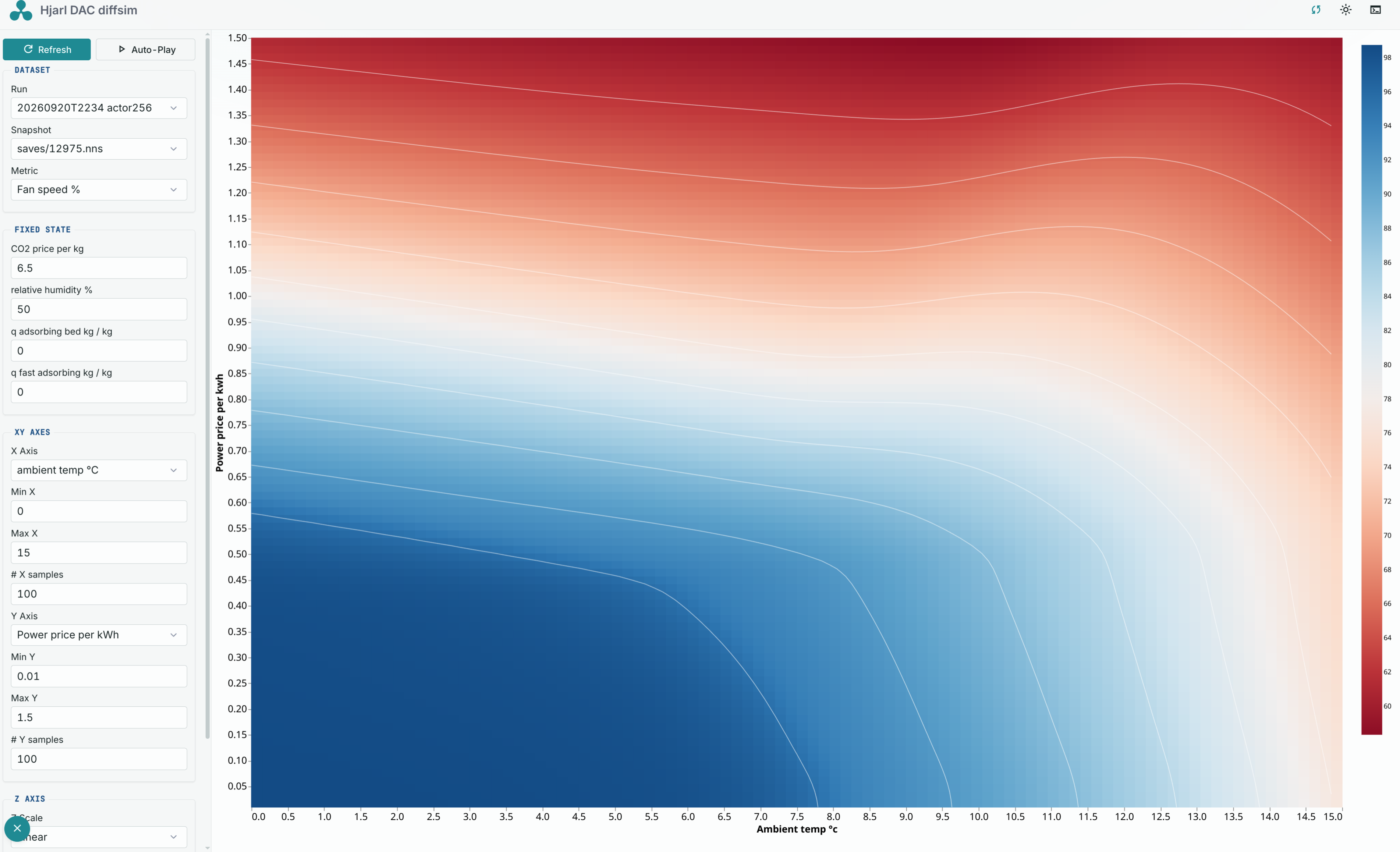
SIMULATOR OUTPUTS
Direct air capture
PILOT · REMOVR / SINTEF / HONEYWELL

Default fan-speed rules optimize only for stability. Trained for 400M simulated hours (10,000 × 40,000h batches), showing meaningful economic uplift across weather and price swings.

LIVE ADVISORY · ON BED CHANGEOVER
  • Inputs: Intake temperature (°C), relative humidity (%), power price (NOK/kWh), and CO₂ price (NOK/kg).
  • Outputs & bounds: 0-100% fan speed, ending state value, and adaptive integration step within changeover and heat exchanger icing limits.
DEPLOYMENT

Runs on a sandboxed on-premise server with revokable certificates and no remote access, advising the Honeywell control system.
Optimal signals use case

⚡ Nodal power shadow pricing: Real-time markets for balancing

heart_plusMitigation (GRADS)
AC POWER FLOW & NODAL SHADOW PRICESopen_in_new
AUTOGRAD-DIFFERENTIABLE AC POWER FLOW

Solves AC power flow for nodal shadow prices and sensitivities (∂loss / ∂control). Built with general autograd rather than hardcoded derivatives, so it integrates directly with other optimizations.

TARGET APPLICATION

Prices voltage, reactive power, active power, and line load bottlenecks in real time.

LIVE INTERACTIVE SHOWCASE

Click any bus or line on the map to pin an override, or toggle Settings to switch scenarios and sensitivity targets.

Launch full-screen AC grid simulator →

Proof of concept

🏭 District heating boiler & storage control

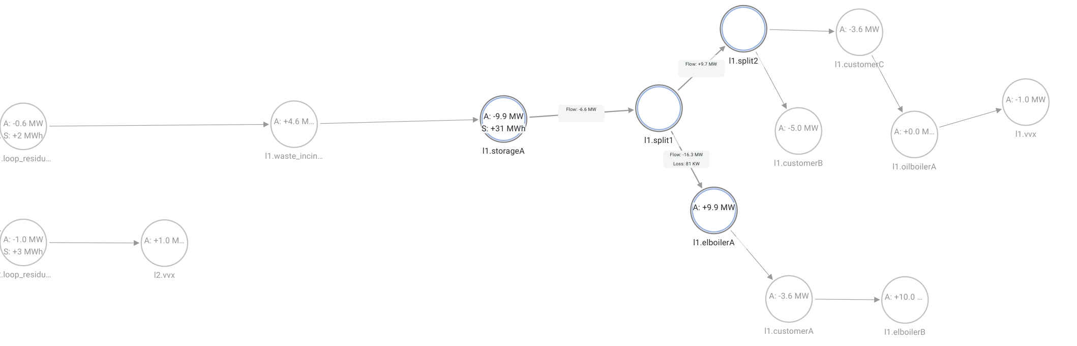
COUPLED BOILERS, STORAGE & LOAD ZONES
District heating topology
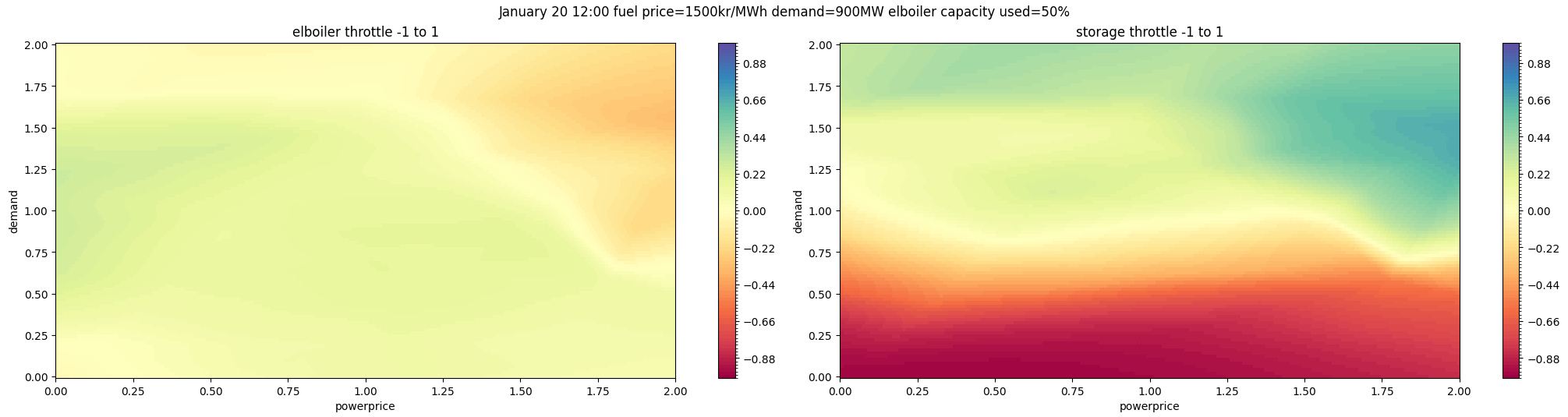
BOILER & STORAGE POLICY SENSITIVITIES
Agent policy sensitivity heatmap
THE CHALLENGE

Coordinate a waste incinerator, oil/electric boilers, and storage buffers against volatile power prices and weather demand.

THE EXECUTION
  • Modeled the thermal grid as a differentiable simulator.
  • Trained across 14,000 parallel simulations (~500,000 hours / 50 years).
THE RESULT

Minimized fuel and peak-capacity tariff costs while meeting 100% of heat demand, using storage buffers optimally across cycles and seasons.
⚛ The core of Hjarl

What Hjarl delivers: A decision policy (π*)

An optimal operating line across shifting terrain

The core of Hjarl

What Hjarl delivers

A decision policy
from an RL-trained agent
trained on a differentiable simulator

A function π*(s) mapping live states to control setpoints.

Decision policy

A decision policy is an optimal operating line across shifting terrain

1 • LIVE DECISION SUPPORT

Maps live states to recommended control setpoints.

2 • BENCHMARKING METRIC

Measures the gap between historical operations and the policy.

3 • TRAINABLE SYSTEM DESIGN

Optimizes physical design parameters alongside control policies across scenarios.

4 • CONTINUOUS IMPROVEMENT LOOP
Operator beats policy ➡ Simulator improves.
Policy beats operator ➡ Procedures improve.

🏃 Looking ahead

Pilot qualification & execution scope

Founder background

The Hjarl thesis at a glance

🏃 Let's build together

The path to running live

1 • WHAT PROBLEMS FIT
  • Can be modeled in a differentiable simulator.
  • Dynamics, distributions, or couplings break convex proxies.
  • Continuous inputs and outputs.
2 • ANCILLARY TASKS
  • Synthetic scenario generation for external drivers.
  • Forecasting models for uncertain inputs.
3 • WHAT IS NEEDED TO START
  • System walkthrough and site visit.
  • Historical series for external drivers.
  • Domain contact for Q&A and benchmark review.
4 • SCOPE OF WORK
  1. Assemble the system simulator (hjarl.systems).
  2. Calibrate external drivers against historical data.
  3. Train the control policy (hjarl.rl).
  4. Deploy a prototype (hjarl.serve + hjarl.dash).
  5. Benchmark against historical operations.

Founder bio

👨‍🔧 Henrik Bakken

EXPERIENCE
2000-05
NTNU · M.Sc. Industrial Economics & Physics.Specialization in statistics and physics; master's thesis at the Norwegian Computing Center on copula theory (paper).
2005-08
The Boston Consulting Group.Consultant.
2008-14
SEB Enskilda Corporate Finance.Shipping & infra, director.
2014-19
Nordic Capital.Private equity, director.
THE PATH TO HJARL
1988
Gaming and tinkering.Got an Amiga in 1988.
2005
Thesis on dependency structures.Realized that causality was vital to learning.
2007
First differentiable simulator.Built to optimize gas flow in pipeline networks.
2015-19
Nighttime AI researcher.Built CNN in 2015 (ResNet), LM in 2018 (BERT), custom CUDA kernels in 2019.
2020
Founded Hjarl.A window to be part of solving learning.

In brief

The Hjarl thesis at a glance

1 • WHY
Real physics isn't a smooth convex bowl.Classical solvers find the exact solution to an imperfect representation. Hjarl finds an imperfect, improvable solution to a near-exact representation.
2 • WHAT
Local control over time, coordinated by signals in space.Policies optimize each asset over time within hard operating limits, while shadow prices coordinate actions across bottlenecks.
3 • HOW
Modular physics simulation with differentiability at its core.The simulator runs physics forward and passes exact gradients backward, while an equilibrium solver updates policies and shadow prices together.
4 • FOR WHOM
For live advice, performance benchmarks, and system design.Advise or automate live operations and benchmark historical decisions. Train physical design parameters alongside control policies ahead of investments.
5 • WHEN
From simulator to sandboxed advisor.Assemble a system simulator, calibrate external drivers, and train a policy, then benchmark against historical operations before deploying in a sandbox.
6 • WHERE
Tested on physical systems that can be differentiated.Hydropower dispatch (Skagerak Energi) and direct air capture (Removr / Honeywell) pilots, plus AC power grid and district heating showcases.

Appendix

RL training, simulation & differentiability (∇f)

Current state of AI control

Fusing RL with classical control theory

RL training

A self-learnt policy requires RL training

CLOSED-LOOP DIFFERENTIABLE RL · POLICY & SIMULATOR
AGENT · DECISION POLICY
u_t = \pi_\theta(s_t)
Updates \theta to maximize \mathbb{E}\!\left[\sum_{t=0}^{T} \gamma^t r_t\right]
STATE & REWARDs_{t+1}, \; r_t(s_t, u_t)+ \nabla f, \; \lambda^*
CONTROL ACTIONu_t \in \mathcal{U}continuous setpoints
SYSTEM · DIFFERENTIABLE SIMULATOR
s_{t+1} = f(s_t, u_t, \xi_t), \quad g(s_t, u_t) \le 0
Physics forward · exact gradients backward
BOTTLENECKS · SAMPLE EFFICIENCY
  • Needs interactive rollouts; static logs are not enough.
  • Sensitive to simulator accuracy and hard bounds.
  • Unsafe to train directly on live industrial hardware.
STRENGTHS · SEQUENTIAL CONTROL
  • Learns multi-step strategies over long horizons.
  • Handles continuous, coupled control and design variables.
  • Purpose-built for physical control, unlike LLMs.

Simulation

Simulation makes RL feasible

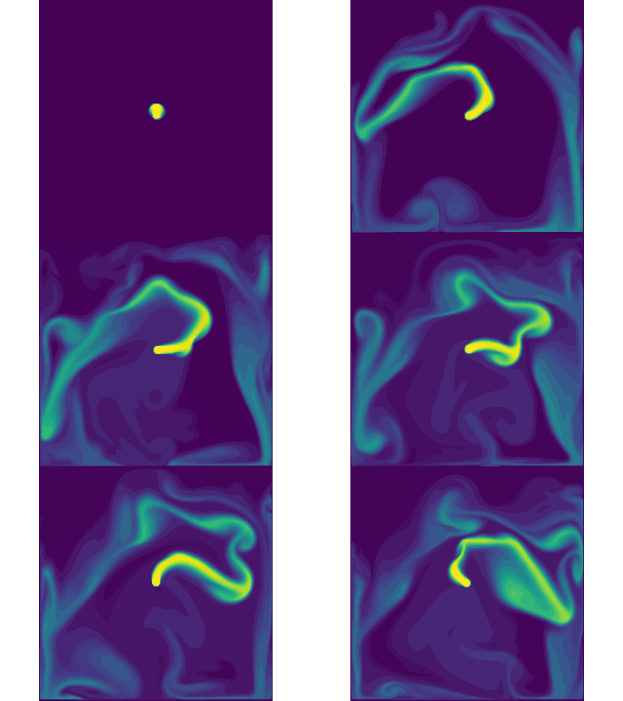
fluidsim
THE DATA LIMIT · HISTORICAL LOGS
  • Logs only show past operator actions, not how the system responds to new policies.
  • Past data goes stale when equipment, capacities, or rules change.
REQUIREMENTS FOR A TRAINING SIMULATOR
  • Physical accuracy across operating regimes and bounds.
  • High GPU throughput (10,000+ parallel rollouts).
  • Modular code that evolves with the system.

Differentiability

Differentiability makes RL scalable

CURSE OF DIMENSIONALITY
  • Standard RL explores by random action noise.
  • Required samples grow exponentially with control dimensions.
EXACT GRADIENTS · ∇f
  • Gradients show directly how each action affects the outcome.
  • Replaces trial-and-error sampling with gradient descent.
  • Cuts sample complexity by orders of magnitude.
EMPIRICAL BENCHMARK · 1st-ORDER GRADIENTS

Exact gradients scale policy learning to 100+ continuous control and design parameters.

Experimentally, our method shows superior asymptotic performance over MFRL baselines in complex locomotion tasks, achieving up to 64% higher reward even when baselines are given 10^6\times more training data. Further, AHAC’s efficient use of first-order gradients enables scaling to high-dimensional motor control tasks with 152 action dimensions.

Adaptive Horizon Actor-Critic (Nvidia Research)

Appendix: The current state of AI control

RL shows promise, but isn't fully researched

Classical vs AI Control
IMPERFECT SOLUTION TO A NEAR-EXACT REPRESENTATION

Complementary to classical solvers and improvable with iterative training, but without formal optimality guarantees.

EXPLORES THE REAL SURFACE INSTEAD OF A CONVEX PROXY

Requires a simulator rather than static historical logs alone.

DECENTRALIZED COORDINATION IS AN OPEN PROBLEM

Nodal market making requires efficient bidders - one must first solve the local agents, and then solve the coordination.

TESTABLE OPTIMUM VIA GRADIENTS AND SHADOW PRICES

Any sub-optimality can be inspected in the gradient - unlike black-box RL.

Appendix: Fusing AI with classical control

Fusing RL with classical control theory

SIMULATORS AS DATA AND GRADIENT GENERATORS
  • Differentiable physics replaces blind sampling with exact gradients.
  • Example: First-order differentiable simulation (Nvidia AHAC) beats model-free RL by 64% with 10^6\times less data.
CLASSICAL METHODS AS YARDSTICKS
  • Classical solvers (like SDDP) handle hard bounds by linking shadow prices (\lambda^*) to the value function.
  • Hjarl brings shadow-price updates into policy learning over long horizons.
EXPLAINABILITY THROUGH MATHEMATICS
  • Shadow prices and gradients make policies auditable (gradients vanish at the optimum).
  • Extends classical principles to non-convex, coupled systems.
CORE CHALLENGES
  • Enforcing hard physical bounds.
  • Optimizing over long horizons.
BENCHMARK DOMAIN: HYDROPOWER
  • Hydropower combines hard bounds, cascades, load-based tariffs, and >1y horizons.
  • Serves as a concrete benchmark against SDDP.